


AIOU 0402 Economics Solved Assignment 1 Spring 2025
AIOU 0402 Assignment 1
Q1. Discuss the scope and nature of economics. Also, define economics in the light of thoughts presented by Professor Robinson.
Economics is a broad and dynamic field that examines how individuals, businesses, and governments allocate resources to satisfy their needs and desires. Its nature is both social and scientific—social because it studies human behavior and interactions, and scientific because it relies on systematic observation, analysis, and theoretical models.
Scope of Economics
The scope of economics extends across various domains:
1. Microeconomics – Focuses on individual consumers, firms, and markets, analyzing factors such as demand, supply, pricing, and production.
2. Macroeconomics – Deals with large-scale economic issues like national income, inflation, employment, and fiscal policies.
3. Development Economics – Examines economic growth, poverty, and strategies for improving living standards.
4. International Economics – Studies trade, globalization, exchange rates, and economic relationships among countries.
5. Public Economics – Explores taxation, government spending, and policies affecting resource allocation.
Nature of Economics
Economics is both a positive and normative science:
1. Positive Economics describes economic phenomena and relationships without making value judgments (e.g., analyzing inflation trends).
2. Normative Economics involves recommendations and policy-making, addressing what "should" be done to improve economic outcomes (e.g., suggesting tax policies).
It is also both a science and an art:
1. As a science, it formulates theories and principles based on empirical observations and data.
2. As an art, it applies those principles to solve economic problems effectively.
Professor Joan Robinson’s Definition of Economics
Joan Robinson, a renowned economist, emphasized a critical and dynamic view of economics. She famously stated that "the purpose of studying economics is not to acquire a set of ready-made answers to economic questions, but to learn how to avoid being deceived by economists." This perspective highlights that economics is not just about memorizing theories but about critically analyzing and questioning economic policies and frameworks.
Robinson was also known for her contributions to imperfect competition theory, where she challenged classical economic models and explored how real-world markets often diverge from the ideal conditions of perfect competition. Her work underscores the importance of understanding economic structures and questioning prevailing assumptions.
Q2.(a Differentiate between utility and satisfaction. Can we measure utility? If yes then explain how?
Utility vs. Satisfaction
Utility and satisfaction are related but distinct concepts in economics and psychology:
1. Utility refers to the perceived usefulness or benefit derived from consuming a good or service. It is an economic concept that helps explain consumer behavior.
2. Satisfaction is a psychological state—an emotional response to consumption. It reflects how pleased or content a person feels after using a product or service.
Can Utility Be Measured?
Yes, utility can be measured, although it's not always straightforward. Economists use two main approaches:
1. Cardinal Utility – Assumes utility can be quantified, measured in numerical terms (e.g., "utils"). However, this method is largely theoretical.
2. Ordinal Utility – Focuses on ranking preferences rather than assigning exact values. It helps economists understand choices without needing a precise measurement.
Methods to Measure Utility:
1. Total Utility – The overall satisfaction gained from consuming a quantity of a good.
2. Marginal Utility – The additional utility received from consuming one more unit of a good.
3. Consumer Choice Models – Surveys and experiments that analyze purchasing behavior to approximate utility.
4. Revealed Preferences – Observing consumer actions rather than relying on direct responses to determine preferences and utility.
In practical terms, utility is difficult to measure directly, as it depends on individual preferences, experiences, and external factors. Economists typically use behavioral analysis, market trends, and experiments to estimate utility rather than measuring it precisely.
Q2.(b Explain the weighted marginal utility and its role in determining the consumer's equilibrium.
Weighted Marginal Utility is an important concept in consumer theory that helps explain how individuals make rational decisions to maximize their satisfaction (utility) given their limited income. It takes into account both the marginal utility (additional satisfaction gained from consuming one more unit of a good) and the price of the good.
Mathematically, weighted marginal utility is expressed as:
MUx / Px and MUy / Py
where:
- MUx and MUy are the marginal utilities of goods X and Y,
- Px and Py are the prices of goods X and Y.
Role in Consumer's Equilibrium
Consumer equilibrium is achieved when a consumer allocates their income in such a way that the ratio of marginal utility to price is equal for all goods they consume. This ensures they derive maximum utility from their budget.
MUx / Px = MUy / Py = ... = MUn / Pn
This principle is known as the Law of Equi-Marginal Utility. It implies:
1. If a consumer finds that the weighted marginal utility of one good is higher than another, they will reallocate their expenditure towards the good providing higher utility until equilibrium is reached.
2. At equilibrium, the consumer cannot improve their overall satisfaction by changing their consumption pattern, given their budget constraint.
3. This ensures optimal resource allocation, preventing wastage of income on goods that do not maximize utility.
In simple terms, a rational consumer distributes their spending in a way that the last unit of money spent on each good provides the same level of satisfaction. This idea helps economists analyze demand patterns and pricing strategies in markets.
Q3.(a What is meant by point elasticity and arc- elasticity? Explain with the help of a diagram and formula.
Point elasticity and arc elasticity are both measures of elasticity, used to calculate the responsiveness of quantity demanded or supplied to changes in price. However, they differ in their approach.
1. Point Elasticity
Point elasticity measures elasticity at a specific point on the demand or supply curve. It is used when analyzing very small changes in price and quantity. The formula for point elasticity is:
E = (dQ/dP) × (P/Q)
Where:
- E = Price elasticity of demand or supply
- dQ/dP = Derivative of quantity with respect to price
- P = Initial price
- Q = Initial quantity
Point elasticity is useful when we have a continuous demand curve and can differentiate the function mathematically.
2. Arc Elasticity
Arc elasticity is used to measure elasticity over a range of prices rather than at a single point. It provides an average elasticity between two points on the demand or supply curve. The formula for arc elasticity is:
E = [(Q2 - Q1) / (Q1 + Q2)] ÷ [(P2 - P1) / (P1 + P2)]
Where:
- E = Arc elasticity
- Q1, Q2 = Initial and final quantity
- P1, P2 = Initial and final price
Arc elasticity is useful when dealing with discrete changes in price and quantity instead of infinitesimally small changes.
Diagram Explanation
- Point Elasticity is calculated at an exact point on the curve.
- Arc Elasticity measures elasticity between two points on the curve.
Q3.(b Given the supply and demand equations:
Qs = 50 + 4p
Qd = 200 - 2p
Estimate
(i) Equilibrium price and quantity.
Step 1: Solve for p
To find the equilibrium price and quantity, we set quantity supplied (Qₛ) equal to quantity demanded (Q_d):
50 + 4p = 200 - 2p
Rearrange the equation:
50 + 4p + 2p = 200
6p = 150
p = 25
So, the equilibrium price is 25.
Step 2: Solve for Q
Substituting p = 25 into either equation:
Qₛ = 50 + 4(25) = 50 + 100 = 150
Q_d = 200 - 2(25) = 200 - 50 = 150
Thus, the equilibrium quantity is 150.
Final Answer:
1. Equilibrium Price = 25
2. Equilibrium Quantity = 150
(ii) Elasticities of demand and supply at equilibrium position.
Step 1: Solve for p
To find the equilibrium price and quantity, we set quantity supplied (Qₛ) equal to quantity demanded (Q_d):
Qₛ = Q_d
Given the equations:
Qₛ = 50 + 4p
Q_d = 200 - 2p
Setting the two equations equal to each other:
50 + 4p = 200 - 2p
Rearrange:
50 + 4p + 2p = 200
6p = 150
p = 25
So, the equilibrium price is 25.
Step 2: Solve for Q
Substituting p = 25 into either equation:
Qₛ = 50 + 4(25) = 50 + 100 = 150
Q_d = 200 - 2(25) = 200 - 50 = 150
Thus, the equilibrium quantity is 150.
Final Answer:
1. Equilibrium Price = 25
2. Equilibrium Quantity = 150
Q4.(a Differentiate between the concepts of average revenue and marginal revenue in the case of perfect competition and imperfect competition with the help of a table and diagrams.
Comparison of AR and MR in Perfect and Imperfect Competition
| Concept | Perfect Competition | Imperfect Competition |
|---|---|---|
| 1. Average Revenue (AR) | AR is constant and equal to price (P). | AR falls as output increases due to the downward-sloping demand curve. |
| 2. Marginal Revenue (MR) | MR is also constant and equal to AR/P. | MR falls faster than AR and lies below the AR curve. |
| 3. Relationship | AR = MR = P (since firms are price takers). | MR is less than AR because firms have price-setting power. |
| 4. Graphical Representation | AR and MR are horizontal and identical. | AR is downward-sloping, and MR is steeper and below AR. |
Diagrams:
1. Perfect Competition: AR and MR curves are horizontal and identical, indicating a price-taking firm.
2. Imperfect Competition: AR curve slopes downward, reflecting a firm’s ability to influence price. MR curve lies below the AR curve and decreases faster.
3. Visual Representation: AR is downward-sloping, and MR is steeper, always lower than AR.
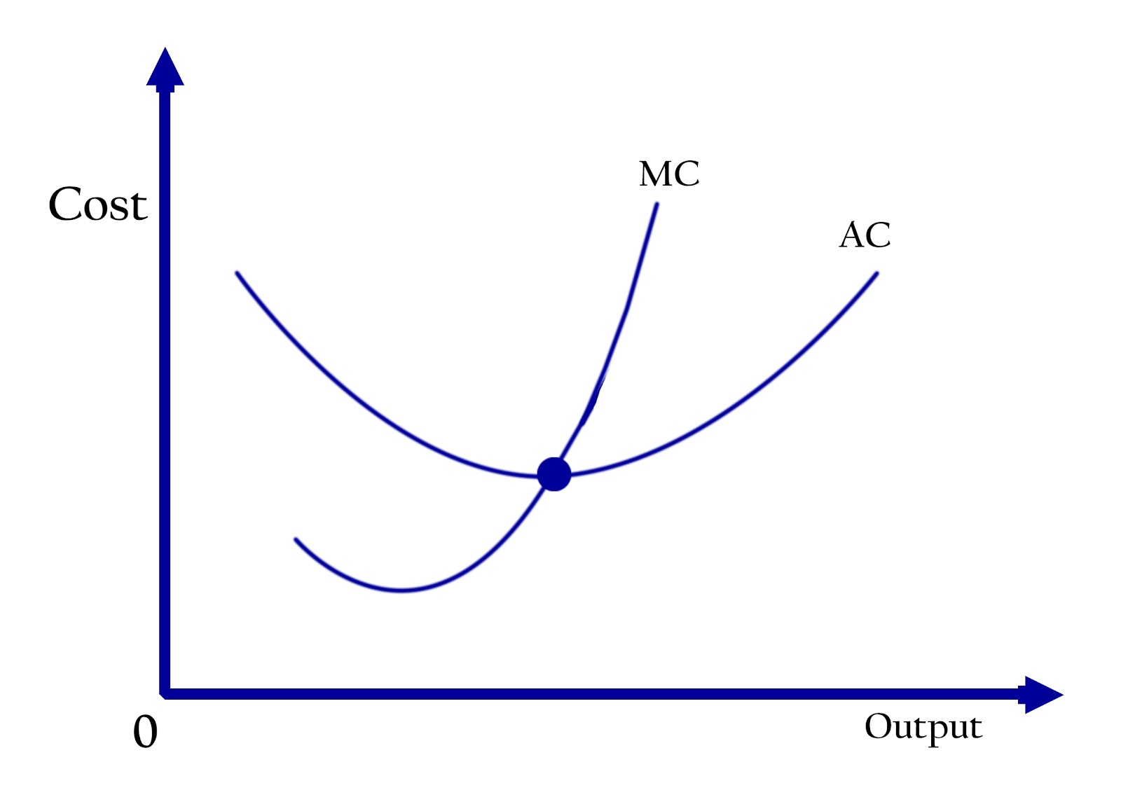
Q4.(b Differentiate between average cost and marginal cost with the help of a table and diagram.
Average cost (AC) refers to the total cost of production divided by the quantity of output, representing the cost per unit produced. It helps businesses assess overall efficiency and pricing strategies. Marginal cost (MC), on the other hand, measures the additional cost incurred when producing one more unit of output, focusing on incremental changes in cost. While average cost provides insight into the broader financial picture, marginal cost plays a crucial role in decision-making, particularly in determining optimal production levels and pricing strategies. Generally, marginal cost influences the behavior of average cost—when MC is below AC, AC decreases, and when MC is above AC, AC rises. Understanding both is essential for effective cost management and maximizing profitability.
Q5. Write a note on the following:
a. Adam Smith’s definition of economics.
Adam Smith, often considered the father of economics, defined economics as the study of wealth—how it is produced, distributed, and consumed. In his seminal work The Wealth of Nations (1776), Smith emphasized that economics is concerned with increasing national wealth through free markets, specialization, and the division of labor. He believed that individuals pursuing their self-interest in a competitive market would unintentionally benefit society as a whole—a concept famously known as the "invisible hand." His definition laid the foundation for classical economics, focusing on production, trade, and the role of markets in economic growth.
b. Law of diminishing marginal utility.
The law of diminishing marginal utility states that as a person consumes more units of a good or service, the additional satisfaction (utility) gained from each extra unit decreases. In other words, the first unit of a product provides the greatest satisfaction, but with each additional unit, the level of enjoyment or benefit progressively declines. For example, imagine eating your favorite dessert—let’s say chocolate cake. The first slice is incredibly satisfying, the second is still enjoyable, but by the third or fourth, you might start feeling full or even uninterested. That decreasing satisfaction with each additional slice is an example of diminishing marginal utility. This principle plays a key role in consumer decision-making, affecting pricing strategies and demand for goods.
c. Income effect and income effect of a price change.
The income effect refers to the change in a consumer's purchasing power when their income changes. When income increases, consumers tend to buy more of most goods, and when income decreases, they reduce their consumption. The income effect of a price change occurs when the price of a good changes, affecting the consumer’s real income or purchasing power. If the price of a good decreases, the consumer feels as though they have more income, enabling them to buy more of that good or other goods. Conversely, if the price rises, the consumer’s effective purchasing power declines, leading to reduced consumption. This effect is particularly strong for normal goods, where demand increases with rising income, and weaker or opposite for inferior goods, where demand may fall as income increases. This concept plays a key role in understanding consumer behavior and market dynamics.
d. Short-run and long- run supply curves.
Short-Run Supply Curve: In the short run, at least one factor of production (such as capital or land) is fixed, meaning firms cannot fully adjust their production capacity. As a result, the short-run supply curve is typically upward-sloping, indicating that firms will produce more as prices rise, but only by adjusting variable inputs like labor and raw materials.
Long-Run Supply Curve: In the long run, all factors of production become variable, allowing firms to enter or exit the market freely and fully adjust their output levels. The long-run supply curve can take different shapes depending on the industry's cost structure:
1. Horizontal – Represents constant-cost industries where input costs remain stable as output expands.
2. Upward-sloping – Occurs in increasing-cost industries, where expanding output leads to higher production costs.
3. Downward-sloping – Found in decreasing-cost industries, where production becomes more efficient as output grows.
The key difference between these curves lies in the flexibility of production. In the short run, firms face constraints due to fixed inputs, whereas in the long run, they can adjust all factors, leading to different market dynamics.
0 Comments:
Post a Comment